Inspired by Petabyte Scale Solutions from CERN
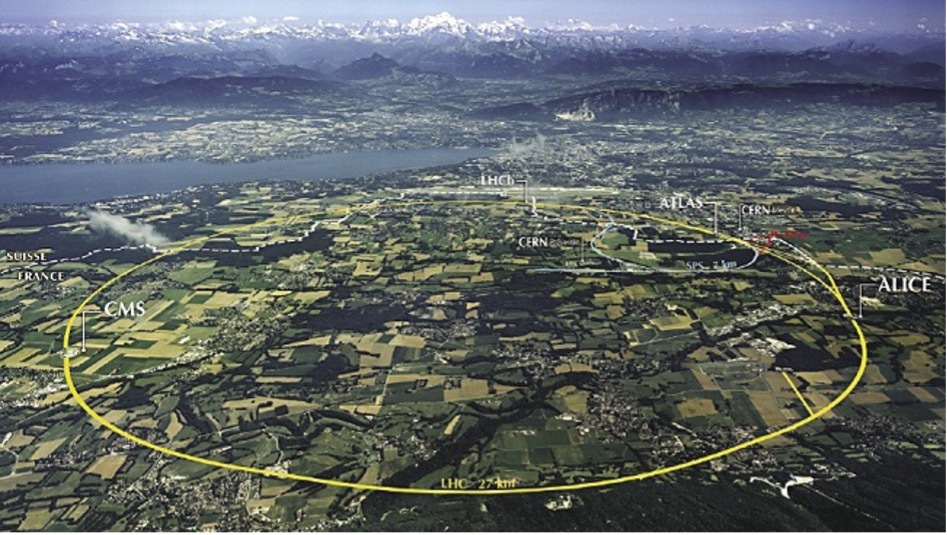
The Large Hadron Collider (LHC) accelerator is the biggest device humankind has ever created. Handling enormous amounts of data it produces has required one of the biggest computational infrastructures on the earth. However, it is quite easy to overwhelm even the best supercomputer with inefficient algorithms that do not correctly utilize the full power of underlying, highly parallel hardware. In this article, I want to share insights born from my meeting with the CERN people, particularly how to validate and improve parallel computing in the data-driven world.
Struggling with data on the scale of megabytes (106 ) to gigabytes (109 ) is the bread and butter for data engineers, data scientists, or machine learning engineers. Moving forward, the terabyte (1012 ) and petabyte (1015 ) scale is becoming increasingly ordinary, and the chances of dealing with it in everyday data-related tasks keep growing. Although the claim “Moore’s law is dead!” is quite a controversial one, the fact is that single-thread performance improvement has slowed down significantly since 2005. This is primarily due to the inability to increase the clock frequency indefinitely. The solution is parallelization – mainly by an increase in the numbers of logical cores available for one processing unit.
Knowing it, the ability to properly parallelize computations is increasingly important.
In a data-driven world, we have a lot of ready-to-use, very good solutions that do most of the parallel stuff on all possible levels for us and expose easy-to-use API. For example, on a large scale, Spark or Metaflow are excellent tools for distributed computing; at the other end, NumPy enables Python users to do very efficient matrix operations on the CPU, something Python is not good at all, by integrating C, C++, and Fortran code with friendly snake_case API. Do you think it is worth learning how it is done behind the scenes if you have packages that do all this for you? I honestly believe this knowledge can only help you use these tools more effectively and will allow you to work much faster and better in an unknown environment.
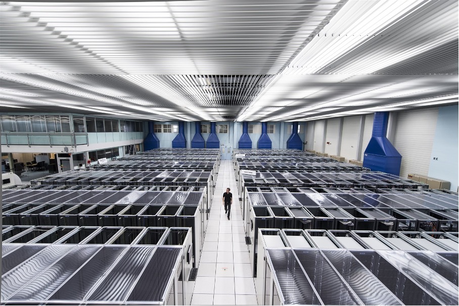
The LHC lies in a tunnel 27 kilometers (about 16.78 mi) in circumference, 175 meters (about 574.15 ft) under a small city built for that purpose on the France–Switzerland border. It has four main particle detectors that collect enormous amounts of data: ALICE, ATLAS, LHCb, and CMS. The LHCb detector alone collects about 40 TB of raw data every second. Many data points come in the form of images since LHCb takes 41 megapixels resolution photos every 25 ns. Such a huge amount of data must be somehow compressed and filtered before permanent storage. From the initial 40 TB/s, only 10G GB/s are saved on disk – the compression ratio is 1:4000!
It was a surprise for me that about 90% of CPU usage in LHCb is done on simulation. One may wonder why they simulate the detector. One of the reasons is that a particle detector is a complicated machine, and scientists at CERN use, i.e., Monte Carlo methods to understand the detector and the biases. Monte Carlo methods can be suitable for massively parallel computing in physics.
Let us skip all the sophisticated techniques and algorithms used at CERN and focus on such aspects of parallel computing, which are common regardless of the problem being solved. Let us divide the topic into four primary areas:
– SIMD,
– multitasking and multiprocessing,
– GPGPU,
– and distributed computing.
The following sections will cover each of them in detail.
SIMD
The acronym SIMD stands for Single Instruction Multiple Data and is a type of parallel processing in Flynn’s taxonomy.
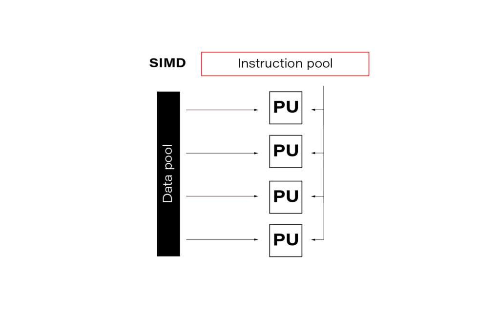
In the data science world, this term is often so-called vectorization. In practice, it means simultaneously performing the same operation on multiple data points (usually represented as a matrix). Modern CPUs and GPGPUs often have dedicated instruction sets for SIMD; examples are SSE and MMX. SIMD vector size has significantly increased over time.
Publishers of the SIMD instruction sets often create language extensions (typically using C/C++) with intrinsic functions or special datatypes that guarantee vector code generation. A step further is abstracting them into a universal interface, e.g., std::experimental::simd from C++ standard library. LLVM’s (Low Level Virtual Machine) libcxx implements it (at least partially), allowing languages based on LLVM (e.g., Julia, Rust) to use IR (Intermediate Representation – code language used internally for LLVM’s purposes) code for implicit or explicit vectorization. For example, in Julia, you can, if you are determined enough, access LLVM IR using macro @code_llvm and check your code for potential automatic vectorization.
In general, there are two main ways to apply vectorization to the program:
– auto-vectorization handled by compilers,
– and rewriting algorithms and data structures.
For a dev team at CERN, the second option turned out to be better since auto-vectorization did not work as expected for them. One of the CERN software engineers claimed that “vectorization is a killer for the performance.” They put a lot of effort into it, and it was worth it. It is worth noting here that in data teams at CERN, Python is the language of choice, while C++ is preferred for any performance-sensitive task.
How to maximize the advantages of SIMD in everyday practice? Difficult to answer; it depends, as always. Generally, the best approach is to be aware of this effect every time you run heavy computation. In modern languages like Julia or best compilers like GCC, in many cases, you can rely on auto-vectorization. In Python, the best bet is the second option, using dedicated libraries like NumPy. Here you can find some examples of how to do it.
Below you can find a simple benchmarking presenting clearly that vectorization is worth attention.
import numpy as np
from timeit import Timer

# Using numpy to create a large array of size 10**6
array = np.random.randint(1000, size=10**6)

# method that adds elements using for loop
def add_forloop():
  new_array = [element + 1 for element in array]

# Method that adds elements using SIMD
def add_vectorized():
  new_array = array + 1

# Computing execution time
computation_time_forloop = Timer(add_forloop).timeit(1)
computation_time_vectorized = Timer(add_vectorized).timeit(1)

# Printing results
print(execution_time_forloop) # gives 0.001202600
print(execution_time_vectorized) # gives 0.000236700
Multitasking and Multiprocessing
Let us start with two confusing yet important terms which are common sources of misunderstanding:
– concurrency: one CPU, many tasks,
– parallelism: many CPUs, one task.
Multitasking is about executing multiple tasks concurrently at the same time on one CPU. A scheduler is a mechanism that decides what the CPU should focus on at each moment, giving the impression that multiple tasks are happening simultaneously. Schedulers can work in two modes:
– preemptive,
– and cooperative.
A preemptive scheduler can halt, run, and resume the execution of a task. This happens without the knowledge or agreement of the task being controlled.
On the other hand, a cooperative scheduler lets the running process decide when the processes voluntarily yield control or when idle or blocked, allowing multiple applications to execute simultaneously.
Switching context in cooperative multitasking can be cheap because parts of the context may remain on the stack and be stored on the higher levels in the memory hierarchy (e.g., L3 cache). Additionally, code can stay close to the CPU for as long as it needs without interruption.
On the other hand, the preemptive model is good when a controlled task behaves poorly and needs to be controlled externally. This may be especially useful when working with external libraries which are out of your control.
Multiprocessing is the use of two or more CPUs within a single Computer system. It is of two types:
– Asymmetric – not all the processes are treated equally; only a master processor runs the tasks of the operating system.
– Symmetric – two or more processes are connected to a single, shared memory and have full access to all input and output devices.
I guess that symmetric multiprocessing is what many people intuitively understand as typical parallelism.
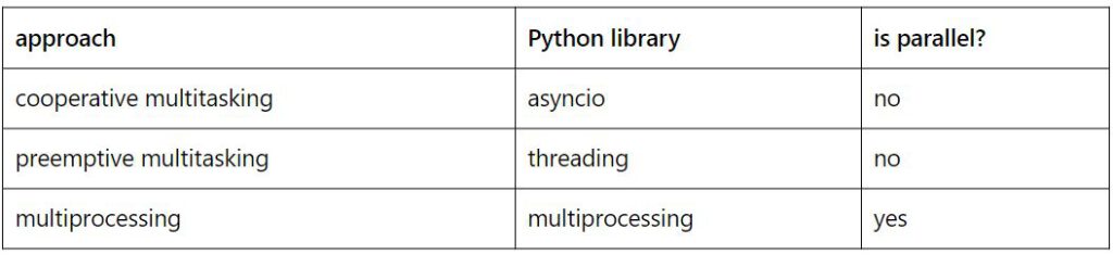
Below are some examples of how to do simple tasks using cooperative multitasking, preemptive multitasking, and multiprocessing in Python. The table below shows which library should be used for each purpose.
– Cooperative multitasking example:
import asyncio
import sys
import time

# Define printing loop
async def print_time():
    while True:
        print(f"hello again [{time.ctime()}]")
        await asyncio.sleep(5)

# Define stdin reader
def echo_input():
    print(input().upper())

# Main function with event loop
async def main():

asyncio.get_event_loop().add_reader(
        sys.stdin,
        echo_input
    )
    await print_time()

# Entry point
asyncio.run(main())
Just type something and admire the uppercase response.
– Preemptive multitasking example:
import threading
import time

# Define printing loop
def print_time():
    while True:
        print(f"hello again [{time.ctime()}]")
        time.sleep(5)

# Define stdin reader
def echo_input():
    while True:
        message = input()
        print(message.upper())

# Spawn threads
threading.Thread(target=print_time).start()
threading.Thread(target=echo_input).start()
The usage is the same as in the example above. However, the program may be less predictable due to the preemptive nature of the scheduler.
– Multiprocessing example:
import time
import sys
from multiprocessing import Process

# Define printing loop
def print_time():
    while True:
        print(f"hello again [{time.ctime()}]")
        time.sleep(5)

# Define stdin reader
def echo_input():
    sys.stdin = open(0)
    while True:
        message = input()
        print(message.upper())

# Spawn processes
Process(target=print_time).start()
Process(target=echo_input).start()
Notice that we must open stdin for the echo_input process because this is an exclusive resource and needs to be locked.
In Python, it may be tempting to use multiprocessing anytime you need accelerated computations. But processes cannot share resources while threads / asyncs can. This is because a process works with many CPUs (with separate contexts) while threads / asyncs are stuck to one CPU. So, you must use synchronization primitives (e.g., mutexes or atomics), which complicates source code. No clear winner here; only trade-offs to consider.
Although that is a complex topic, I will not cover it in detail as it is uncommon for data projects to work with them directly. Usually, external libraries for data manipulation and data modeling encapsulate the appropriate code. However, I believe that being aware of these topics in contemporary software is particularly useful knowledge that can significantly accelerate your code in unconventional situations.
You may find other meanings of the terminology used here. After all, it is not so important what you call it but rather how to choose the right solution for the problem you are solving.
GPGPU
General-purpose computing on graphics processing units (GPGPU) utilizes shaders to perform massive parallel computations in applications traditionally handled by the central processing unit.
In 2006 Nvidia invented Compute Unified Device Architecture (CUDA) which soon dominated the machine learning models acceleration niche. CUDA is a computing platform and offers API that gives you direct access to parallel computation elements of GPU through the execution of computer kernels.
Returning to the LHCb detector, raw data is initially processed directly on CPUs operating on detectors to reduce network load. But the whole event may be processed on GPU if the CPU is busy. So, GPUs appear early in the data processing chain.
GPGPU’s importance for data modeling and processing at CERN is still growing. The most popular machine learning models they use are decision trees (boosted or not, sometimes ensembled). Since deep learning models are harder to use, they are less popular at CERN, but their importance is still rising. However, I am quite sure that scientists worldwide who work with CERN’s data use the full spectrum of machine learning models.
To accelerate machine learning training and prediction with GPGPU and CUDA, you need to create a computing kernel or leave that task to the libraries’ creators and use simple API instead. The choice, as always, depends on what goals you want to achieve.
For a typical machine learning task, you can use any machine learning framework that supports GPU acceleration; examples are TensorFlow, PyTorch, or cuML, whose API mirrors Sklearn’s. Before you start accelerating your algorithms, ensure that the latest GPU driver and CUDA driver are installed on your computer and that the framework of choice is installed with an appropriate flag for GPU support. Once the initial setup is done, you may need to run some code snippet that switches computation from CPU (typically default) to GPU. For instance, in the case of PyTorch, it may look like that:
import torch

torch.cuda.is_available()
def get_default_device():
    if torch.cuda.is_available():
        return torch.device('cuda')
    else:
        return torch.device('cpu')
device = get_default_device()
device
Depending on the framework, at this point, you can process as always with your model or not. Some frameworks may require, e. g. explicit transfer of the model to the GPU-specific version. In PyTorch, you can do it with the following code:
net = MobileNetV3()
net = net.cuda()
At this point, we usually should be able to run .fit(), .predict(), .eval(), or something similar. Looks simple, doesn’t it?
Writing a computing kernel is much more challenging. However, there is nothing special about computing kernel in this context, just a function that runs on GPU.
Let’s switch to Julia; it is a perfect language for learning GPU computing. You can get familiar with why I prefer Julia for some machine learning projects here. Check this article if you need a brief introduction to the Julia programming language.
Data structures used must have an appropriate layout to enable performance boost. Computers love linear structures like vectors and matrices and hate pointers, e. g. in linked lists. So, the very first step to talking to your GPU is to present a data structure that it loves.
using Cuda

# Data structures for CPU
N = 2^20
x = fill(1.0f0, N)  # a vector filled with 1.0
y = fill(2.0f0, N)  # a vector filled with 2.0

# CPU parallel adder
function parallel_add!(y, x)
    Threads.@threads for i in eachindex(y, x)
        @inbounds y[i] += x[i]
    end
    return nothing
end

# Data structures for GPU
x_d = CUDA.fill(1.0f0, N)
# a vector stored on the GPU filled with 1.0
y_d = CUDA.fill(2.0f0, N)
# a vector stored on the GPU filled with 2.0

# GPU parallel adder
function gpu_add!(y, x)
    CUDA.@sync y .+= x
    return
end
GPU code in this example is about 4x faster than the parallel CPU version. Look how simple it is in Julia! To be honest, it is a kernel imitation on a very high level; a more real-life example may look like this:
function gpu_add_kernel!(y, x)
    index = (blockIdx().x - 1) * blockDim().x + threadIdx().x
    stride = gridDim().x * blockDim().x
    for i = index:stride:length(y)
        @inbounds y[i] += x[i]
    end
    return
end
The CUDA analogs of threadid and nthreads are called threadIdx and blockDim. GPUs run a limited number of threads on each streaming multiprocessor (SM). The recent NVIDIA RTX 6000 Ada Generation should have 18,176 CUDA Cores (streaming processors). Imagine how fast it can be even compared to one of the best CPUs for multithreading AMD EPYC 7773X (128 independent threads). By the way, 768MB L3 cache (3D V-Cache Technology) is amazing.
Distributed Computing
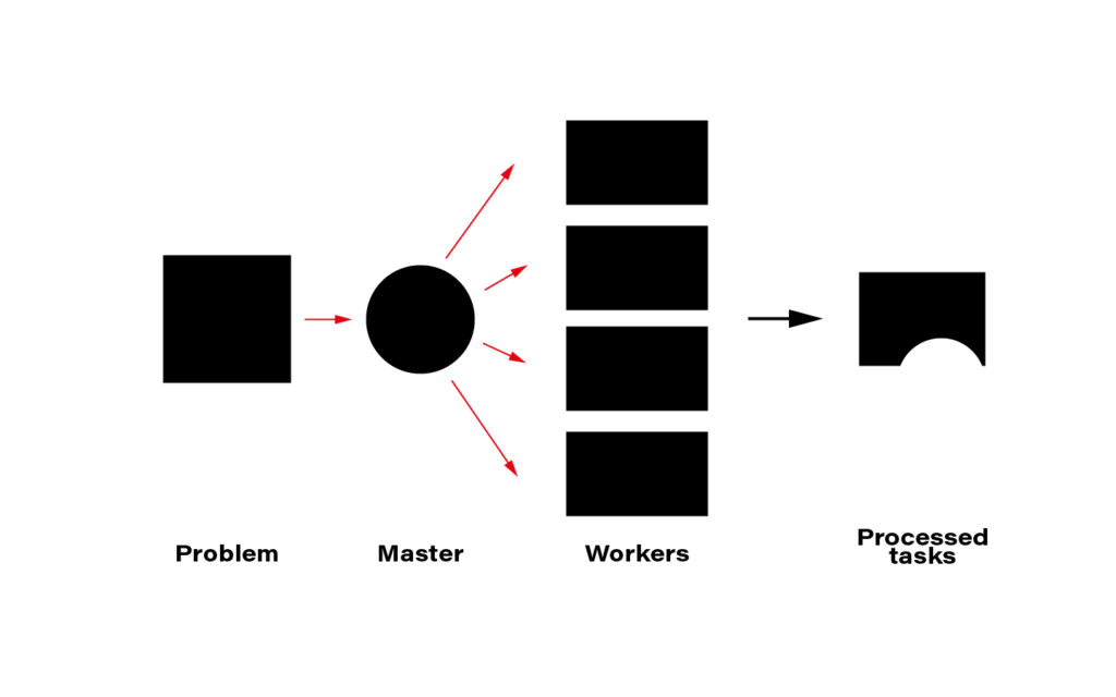
The term distributed computing, in simple words, means the interaction of computers in a network to achieve a common goal. The network elements communicate with each other by passing messages (welcome back cooperative multitasking). Since every node in a network usually is at least a standalone virtual machine, often separate hardware, computing may happen simultaneously. A master node can split the workload into independent pieces, send them to the workers, let them do their job, and concatenate the resulting pieces into the eventual answer.
The computer case is the symbolic border line between the methods presented above and distributed computing. The latter must rely on a network infrastructure to send messages between nodes, which is also a bottleneck. CERN uses thousands of kilometers of optical fiber to create a huge and super-fast network for that purpose. CERN’s data center offers about 300,000 physical and hyper-threaded cores in a bare-metal-as-a-service model running on about seventeen thousand servers. A perfect environment for distributed computing.
Moreover, since most data CERN produces is public, LHC experiments are completely international – 1400 scientists, 86 universities, and 18 countries – they all create a computing and storage grid worldwide. That enables scientists and companies to run distributed computing in many ways.
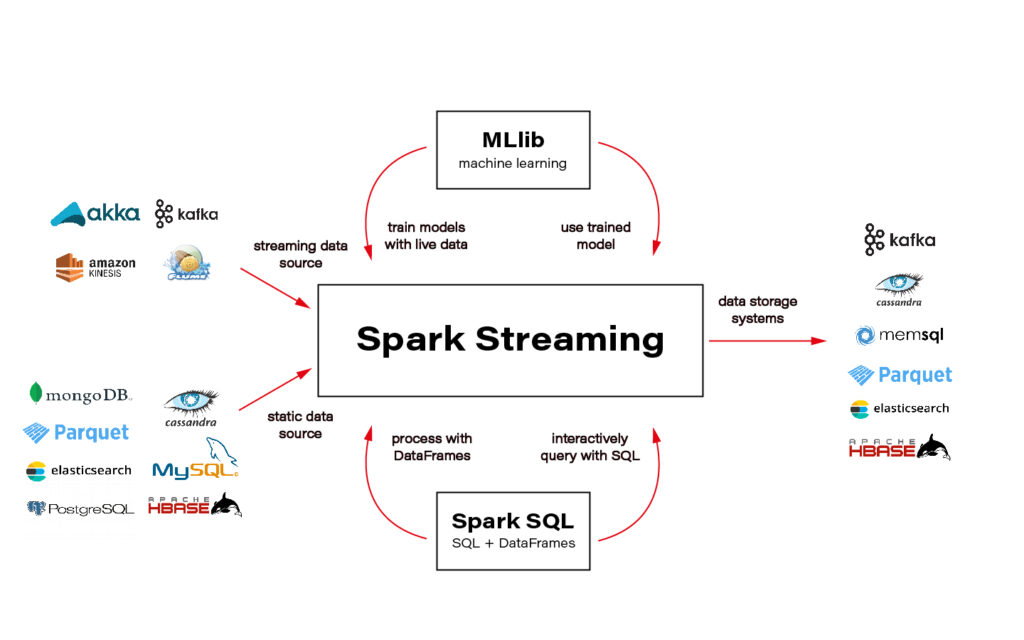
Although this is important, I will not cover technologies and distributed computing methods here. The topic is huge and very well covered on the internet. An excellent framework recommended and used by one of the CERN scientists is Spark + Scala interface. You can solve almost every data-related task using Spark and execute the code in a cluster that distributes computation on nodes for you.
Ok, the only piece of advice: be aware of how much data you send to the cluster – transferring big data can ruin all the profit from distributing the calculations and cost you a lot of money.
Another excellent tool for distributed computation on the cloud is Metaflow. I wrote two articles about Metaflow: introduction and how to run a simple project. I encourage you to read and try it.
Conclusions
CERN researchers have convinced me that wise parallelization is crucial to achieving complex goals in the contemporary Big Data world. I hope I managed to infect you with this belief. Happy coding!
Source link