LangChain is one of the hottest development platforms for creating applications that use generative AI—but it’s only available for Python and JavaScript. What to do if you’re an R programmer who wants to use LangChain?
Fortunately, you can do lots of useful things in LangChain with pretty basic Python code. And, thanks to the reticulate R package, R and RStudio users can write and run Python in the environment they’re comfortable with—including passing objects and data back and forth between Python and R.
In this LangChain tutorial, I’ll show you how to work with Python and R to access LangChain and OpenAI APIs. This will let you use a large language model (LLM)—the technology behind ChatGPT—to query ggplot2‘s 300-page PDF documentation. Our first sample query: “How do you rotate text on the x-axis of a graph?”
Here’s how the process breaks down, step by step:
- If you haven’t already, set up your system to run Python and
reticulate. - Import the
ggplot2PDF documentation file as a LangChain object with plain text. - Split the text into smaller pieces that can be read by a large language model, since those models have limits to how much they can read at once. The 300 pages of text will exceed OpenAI’s limits.
- Use an LLM to create “embeddings” for each chunk of text and save them all in a database. An embedding is a string of numbers that represents the semantic meaning of text in multidimensional space.
- Create an embedding for the user’s question, then compare the question embedding to all the existing ones from the text. Find and retrieve the most relevant text pieces.
- Feed only those relevant portions of text to an LLM like GPT-3.5 and ask it to generate an answer.
If you’re going to follow the examples and use the OpenAI APIs, you’ll need an API key. You can sign up at platform.openai.com. If you’d rather use another model, LangChain has components to build chains for numerous LLMs, not only OpenAI’s, so you’re not locked in to one LLM provider.
LangChain has the components to handle most of these steps easily, especially if you’re satisfied with its defaults. That’s why it’s becoming so popular.
Let’s get started.
Step 1: Set up your system to run Python in RStudio
If you already run Python and reticulate, you can skip to the next step. Otherwise, let’s make sure you have a recent version of Python on your system. There are many ways to install Python, but simply downloading from python.org worked for me. Then, install the reticulate R package the usual way with install.packages("reticulate").
If you’ve got Python intalled but reticulate can’t find it, you can use the command use_python("/path/to/your/python").
It’s good Python practice to use virtual environments, which allow you to install package versions that won’t conflict with the requirements of other projects elsewhere on your system. Here’s how to create a new Python virtual environment and use R code to install the packages you’ll need:
library(reticulate)
virtualenv_create(envname = "langchain_env", packages = c( "langchain", "openai", "pypdf", "bs4", "python-dotenv", "chromadb", "tiktoken")) # Only do this once
Note that you can name your environment whatever you like. If you need to install packages after creating the environment, use py_install(), like this:
py_install(packages = c( "langchain", "openai", "pypdf", "bs4", "python-dotenv", "chromadb", "tiktoken"), envname = "langchain_env")
As in R, you should only need to install packages once, not every time you need to use the environment. Also, don’t forget to activate your virtual environment, with
use_virtualenv("langchain_env")
You’ll do this each time you come back to the project and before you start running Python code.
You can test whether your Python environment is working with the obligatory
reticulate::py_run_string('
print("Hello, world!")
')
You can set your OpenAI API key with a Python variable if you like. Since I already have it in an R environment variable, I usually set the OpenAI API key using R. You can save any R variable to a Python-friendly format with reticulate’s r_to_py() function, including environment variables:
api_key_for_py <- r_to_py(Sys.getenv("OPENAI_API_KEY"))
That takes the OPENAI_API_KEY environment variable, ensures it’s Python-friendly, and stores it in a new variable: api_key_for_py (again, the name can be anything).
At last, we’re ready to code!
Step 2: Download and import the PDF file
I’m going to create a new docs subdirectory of my main project directory and use R to download the file there.
# Create the directory if it doesn't exist
if(!(dir.exists("docs"))) {
  dir.create("docs")
}

# Download the file
download.file("https://cran.r-project.org/web/packages/ggplot2/ggplot2.pdf", destfile = "docs/ggplot2.pdf", mode = "wb")
Next comes the Python code to import the file as a LangChain document object that includes content and metadata. I’ll create a new Python script file called prep_docs.py for this work. I could keep running Python code right within an R script by using the py_run_string() function as I did above. However, that’s not ideal if you’re working on a larger task, because you lose out on things like code completion.
Critical point for Python newbies: Don’t use the same name for your script file as a Python module you’ll be loading! In other words, while the file doesn’t have to be called prep_docs.py, don’t name it, say, langchain.py if you will be importing the langchain package! They’ll conflict. This isn’t an issue in R.
Here’s the first part of my new prep_docs.py file:
# If running from RStudio, remember to first run in R:
# library(reticulate)
# use_virtualenv("the_virtual_environment_you_set_up")
# api_key_py <- r_to_py(Sys.getenv("OPENAI_API_KEY"))
from langchain.document_loaders import PyPDFLoader
my_loader = PyPDFLoader('docs/ggplot2.pdf')
# print(type (my_loader))
all_pages = my_loader.load()
# print(type(all_pages))
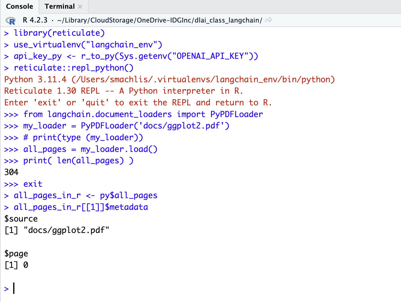
print( len(all_pages) )
This code first imports the PDF document loader PyPDFLoader. Next, it creates an instance of that PDF loader class. Then, it runs the loader and its load method, storing the results in a variable named all_pages. That object is a Python list.
I’ve included some commented lines that will print the object types if you’d like to see them. The final line prints the length of the list, which in this case is 304, one for each page in the PDF.
You can click the source button in RStudio to run a full Python script. Or, highlight some lines of code and only run those, just as with an R script. The Python code looks a little different when running than R code does, since it opens a Python interactive REPL session right within your R console. You’ll be instructed to type exit or quit (without parentheses) to exit and return to your regular R console when you’re finished.
 Sharon Machlis for IDG
You can examine the all_pages Python object in R by using reticulate‘s py object. The following R code stores that Python all_pages object into an R variable named all_pages_in_r (you can call it anything you’d like). You can then work with the object like any other R object. In this case, it’s a list.
all_pages_in_r <- py$all_pages
# Examples:
all_pages_in_r[[1]]$metadata # See metadata in the first item
nchar(all_pages_in_r[[100]]$page_content) # Count number of characters in the 100th item
Step 3: Split the document into pieces
LangChain has several transformers for breaking up documents into chunks, including splitting by characters, tokens, and markdown headers for markdown documents. One recommended default is the RecursiveCharacterTextSplitter, which “recursively tries to split by different characters to find one that works.” Another popular option is the CharacterTextSplitter, which is designed to have the user set its parameters.
You can set this splitter’s maximum text-chunk size, whether it should count by characters or LLM tokens (tokens are typically one to four characters), and how much the chunks should overlap. I hadn’t thought about the need to have text chunks overlap until I began using LangChain, but it makes sense unless you can separate by logical pieces like chapters or sections separated by headers. Otherwise, your text may get split mid-sentence, and an important piece of information could end up divided between two chunks, without the full meaning being clear in either.
You can also select what separators you want the splitter to prioritize when it divvies up your text. CharacterTextSplitter‘s default is to split first on two new lines (nn), then one new line, a space, and finally no separator at all.
The code below imports my OpenAI API key from the R api_key_for_py variable by using reticulate’s r object inside of Python. It also loads the openai Python package and LangChain’s Recursive Character Splitter, creates an instance of the RecursiveCharacterTextSplitter class, and runs that instance’s split_documents() methods on the all_pages chunks.
import openai
openai.api_key = r.api_key_for_py
from langchain.text_splitter import RecursiveCharacterTextSplitter
my_doc_splitter_recursive = RecursiveCharacterTextSplitter()
my_split_docs = my_doc_splitter_recursive.split_documents(all_pages)
Again, you can send these result to R with R code such as:
my_split_docs <- py$my_split_docs
Are you wondering what is the maximum number of characters in a chunk? I can check this in R with a little custom function for the list:
get_characters <- function(the_chunk) {
x <- nchar(the_chunk$page_content)
return(x)
}

purrr::map_int(my_split_docs, get_characters) |>
max()
That generated 3,985, so it looks like the default chunk maximum is 4,000 characters.
If I wanted smaller text chunks, I’d first try the CharacterTextSplitter and manually set chunk_size to less than 4,000, such as
chunk_size = 1000
chunk_overlap = 150
from langchain.text_splitter import CharacterTextSplitter
c_splitter = CharacterTextSplitter(chunk_size=chunk_size, chunk_overlap=chunk_overlap, separator=" ")
c_split_docs = c_splitter.split_documents(all_pages)
print(len(c_split_docs)) # To see in Python how many chunks there are now
I can inspect the results in R as well as Python:
c_split_docs <- py$c_split_docs
length(c_split_docs)
That code generated 695 chunks with a maximum size of 1,000.
What’s the cost?
Before going further, I’d like to know if it’s going to be insanely expensive to generate embeddings for all those chunks. I’ll start with the default recursive splitting’s 306 items. I can calculate the total number of characters in those chunks on the R object with:
purrr::map_int(my_split_docs, get_characters) |>
  sum()
The answer is 513,506. Conservatively estimating two characters per token, that would work out to around 200,000.
If you want to be more exact, the TheOpenAIR R package has a count_tokens() function (make sure to install both that and purrr to use the R code below):
purrr::map_int(my_split_docs, ~ TheOpenAIR::count_tokens(.x$page_content)) |>
   sum()
That code shows 126,343 tokens.
How much would that cost? OpenAI’s model designed to generate embeddings is ada-2. As of this writing ada-2 costs $0.0001 for 1K tokens, or about 1.3 cents for 126,000. That’s within budget!
Step 4: Generate embeddings
LangChain has pre-made components to both create embeddings from text chunks and store them. For storage, I’ll use one of the simplest options available in LangChain: Chroma, an open-source embedding database that you can use locally.
First, I’ll create a subdirectory of my docs directory with R code just for the database, since it’s suggested to not have anything but your database in a Chroma directory. This is R code:
if(!dir.exists("docs/chroma_db")) {
  dir.create("docs/chromaba_db")
}
Below is some Python code to generate the embeddings using LangChain’s OpenAIEmbeddings. That currently defaults to OpenAI’s ada-2 model, so you don’t need to specify it. LangChain supports a number of other LLMs with its Embeddings class, though, including Hugging Face Hub, Cohere, Llama-cpp, and Spacy.
The Python code below is slightly modified from DeepLearning.AI’s LangChain Chat with Your Data online tutorial.
from langchain.embeddings.openai import OpenAIEmbeddings
embed_object = OpenAIEmbeddings()

from langchain.vectorstores import Chroma
chroma_store_directory = "docs/chroma_db"

vectordb = Chroma.from_documents(
    documents=my_split_docs,
    embedding=embed_object,
    persist_directory=chroma_store_directory
)

# Check how many embeddings were created
print(vectordb._collection.count())
Note the underscore in _collection.count()!
I see 306 embeddings, the same number as my ggplot2 text chunks.
Another note for Python newbies: Indentation matters in Python. Make sure non-indented lines have no spaces before them and indented lines all use the same number of indent spaces.
It appears on my system that this code saved the data to disk. However, the tutorial says we should run the following Python code to save the embeddings for later use. I’ll do that, too, since I don’t want to have to re-generate embeddings unless the document changes.
vectordb.persist()
We’re now done with prepping the documents for querying. I’ll create a new file, qanda.py, to use the vector embeddings we’ve created.
Step 5: Embed the user query and find document chunks
Now it’s time to ask a question, generate embeddings for that question, and retrieve the documents that are most relevant to the question based on the chunks’ embeddings.
LangChain gives us several ways to do all of this in a single line of code, thanks to the vectordb object’s built-in methods. Its similarity_search() method does a straightforward calculation of vector similarities and returns the most similar text chunks.
There are several other ways to do this, though, including max_marginal_relevance_search(). The idea behind that one is you don’t necessarily want three text chunks that are almost the same. Maybe you’d end up with a richer response if there was a little diversity in the text to get additional useful information. So, max_marginal_relevance_search() retrieves a few more relevant texts than you actually plan to pass to the LLM for an answer (you decide how many more). It then selects the final text pieces, incorporating some degree of diversity.
You specify how many relevant text chunks you’d like similarity_search() to return with its k argument. For max_marginal_relevance(), you specify how many chunks should initially be retrieved with fetch_k, and how many final text pieces you want the LLM to look through for its answer with k.
I don’t want to run the document prep file if the documents haven’t changed, so I’ll first load the necessary packages and environment variables (i.e., my OpenAI API key) in the new qanda.py file, as I did before using doc_prep.py. Then, I’ll load my chromadb vector database:
# If running from RStudio, remember to first run in R:
# library(reticulate)
# use_virtualenv("the_virtual_environment_you_set_up")
# api_key_py <- r_to_py(Sys.getenv("OPENAI_API_KEY"))

import openai
openai.api_key = r.api_key_for_py
from langchain.embeddings.openai import OpenAIEmbeddings
embed_object = OpenAIEmbeddings()

from langchain.vectorstores import Chroma
chroma_store_directory = "docs/chroma_db"
vectordb = Chroma(persist_directory=chroma_store_directory,
                  embedding_function=embed_object)
Next, I’ll hard-code a question and retrieve the relevant documents. Note that I can retrieve the documents with a single line of code:
my_question = "How do you rotate text on the x-axis of a graph?"
# For straightforward similarity searching
sim_docs = vectordb.similarity_search(my_question)

# For maximum marginal relevance search retrieving 5 possible chunks and choosing 3 finalists:
mm_docs = vectordb.max_marginal_relevance_search(my_question, k = 3, fetch_k = 5)
If you want to view the retrieved document pieces, you can print them in Python with something like the following:
for doc in mm_docs:
    print(doc.page_content)

for doc in sim_docs:
    print(doc.page_content)
Note the indents as part of the for loops.
You can also view their metadata with:
for doc in mm_docs:
    print(doc.metadata)

for docs in sim_docs:
    print(docs.metadata)
As with the other objects, you can also look at these in R:
mm_relevant <- py$mm_docs
sim_relevant <- py$sim_docs
I’m not sure why models sometimes return four documents when I ask for three, but that shouldn’t be a problem—unless it’s too many tokens for the LLM when it goes through the text to generate a response.
Step 6: Generate your answer
It’s now time to ask an LLM like GPT-3.5 to generate a written response to the user’s question based on the relevant documents. You can do that with LangChain’s RetrievalQA function.
I suggest first trying LangChain’s default template for this, which is easy and often works well for prototyping or your own use:
# Set up the LLM you want to use, in this example OpenAI's gpt-3.5-turbo
from langchain.chat_models import ChatOpenAI
the_llm = ChatOpenAI(model_name="gpt-3.5-turbo", temperature=0)

# Create a chain using the RetrievalQA component
from langchain.chains import RetrievalQA
qa_chain = RetrievalQA.from_chain_type(the_llm,retriever=vectordb.as_retriever())

# Run the chain on the question, and print the result
print(qa_chain.run(my_question))
The AI sent back the following response:
To rotate text on the x-axis of a graph, you can use the `theme()` function in ggplot2. Specifically, you can use the `axis.text.x` argument to modify the appearance of the x-axis text. Here is an example:

```R
library(ggplot2)

# Create a basic scatter plot
p <- ggplot(mtcars, aes(x = mpg, y = wt)) +
  geom_point()

# Rotate x-axis text by 45 degrees
p + theme(axis.text.x = element_text(angle = 45, hjust = 1))
```

In this example, the `angle` argument is set to 45, which rotates the x-axis text by 45 degrees. The `hjust` argument is set to 1, which aligns the text to the right. You can adjust the angle and alignment values to achieve the desired rotation and alignment of the x-axis text.
Looks correct!
Now that the chain is set up, you can run it on other questions with just one command using an R script:
py_run_string('
print(qa_chain.run("How can I make a bar chart where the bars are steel blue?"))
')
Here’s the response:
```R
library(ggplot2)

# Create a bar chart with steel blue bars
p <- ggplot(mtcars, aes(factor(cyl)))
p + geom_bar(fill = "steelblue")
```

In this example, we use the `fill` aesthetic to specify the color of the bars as "steelblue". You can adjust the color to your preference by changing the color name or using a hexadecimal color code.
This is a better answer than I sometimes receive when asking ChatGPT 3.5 the same question. (Sometimes the code it sends back doesn’t actually work.)
You might also want to confirm that the answers aren’t being pulled from the general ChatGPT knowledge base, but are really coming from the document you uploaded. To find out, you could ask something completely unrelated to ggplot2 that wouldn’t be in the documentation:
py_run_string('
print(qa_chain.run("What is the capital of Australia?"))
')
You should get back:
I don't know.
“I don’t know” may be a little terse if you’re creating an application for wider use. You can check out the LangChain documentation if you’d like to customize the default template. Personalizing the response makes sense if you are creating an application for more than yourself or a small team .
Template tweaks is one area where LangChain may feel overly complex—it can take multiple lines of code to implement small changes to a template. However, that’s a risk in using any opinionated framework, and it’s up to each developer to decide if the project’s overall benefits are worth such costs. While it is enormously popular, not everyone is a fan of LangChain.
What else can you do with LangChain?
The easiest addition to the application so far would be to include more documents. LangChain has a DirectoryLoader to make this straightforward. If you’re searching across multiple documents, you might want to know which docs were used to generate the response. You can add the return_source_documents=True argument to RetrievalQA, like this:
qa_chain = RetrievalQA.from_chain_type(the_llm,retriever=vectordb.as_retriever(), return_source_documents=True)
my_result = qa_chain({"query": my_question})
print(my_result['result'])
The code is initially only useful to run locally for a single user, but it could be the logic basis for an interactive web application using a framework like Streamlit or Shiny for Python. Or, you combine Python and R, send the LLM’s final answer back to R, and create an application using the Shiny R web framework (although I’ve discovered that deploying a Shiny app with both Python and R is somewhat complicated).
Note, too, that this application isn’t technically a “chatbot” since it won’t remember your previous questions. So, you couldn’t have a “conversation” such as “How can I change the size of a graph’s headline text?” followed by “What about the legend?” You’d have to spell out each new question completely, such as “How do you change the size of a legend’s headline?”
However, you could add memory to the application to turn it into a chatbot with LangChain’s ConversationBufferMemory.
Further resources
To learn more about LangChain, in addition to the LangChain documentation, there is a LangChain Discord server that features an AI chatbot, kapa.ai, that can query the docs.
I’ve worked through about one-third of Udemy’s Develop LLM powered applications with LangChain by Eden Marco, and so far it’s been helpful. While that course says you should be “proficient in Python,” I think knowing other programming languages along with willingness to do plenty of searching/ChatGPT-ing should be enough.
For info on Streamlit and LangChain, there are several tutorials on the Streamlit site, including LangChain tutorial #1: Build an LLM-powered app in 18 lines of code.
Finally, Posit’s Winston Chang is working on an experimental chatstream package for Shiny Python that will include a “streaming” interface so the LLM response appears gradually by character or word, the way ChatGPT’s does, instead of all at once as in these examples.
Copyright © 2023 IDG Communications, Inc.
Source link